Distributed Training
Training advanced neural networks, particularly deep learning models such as transformers, presents significant computational challenges. These sophisticated models require substantial computational power, often exceeding the capabilities of the single GPU machine. The primary hurdles stem from the immense number of parameters that need to be calculated and updated during the training process. This not only demands extensive GPU memory but also nencassitates the use of large batch sizes to achieve efficient learning and convergence.
As the complexity of models grows, So does the need for more advanced hardware accelerators. GPUs (Graphics Processing Units) have become essential in the field of deep learning due to their ability to handle parallel computations effectively. These accelerators significantly reduce training time by distributing the computational load across multiple cores. GPUs whith their high throughput, are particularly well-suited for tasks involving large batch sizes and extensive data parallelism. These accelerators are invaluable for training extremely large models that would otherwise be infeasible on traditional hardware.
The necassity for such powerful accelerators highlights the ever growing demands of deep learning technologies and sets the stage for exploring distributed training methods, which aim to further amplify the capabilities of induvidual training sessions by leveraging multiple GPUs or TPUs simultaneosly.
Essentials of distributed Training#
Lets have a refresher on how deep learning models work. Deep Learning models operate on a mechanism known as gradient descent, a fundamental technique used to optimize these models by mimicking a data representations. During the training process, a model adjusts its internal parameters or weights based on the difference between its predictions and the actual outputs. This difference is qualified through a loss function, which measures the model performance. The backward pass of training involves updating these weights by calculating gradients, which are essentially directions and magnitudes for improving model predictions.
To manage these gradients, optimizers like Adam are employed. These optimizers not only update the weights based on the gradients but also keep track of past gradient values to make informed adjustments, enhancing the efficiency and stability of the learning process.
In the context of distributed deep learning, the training process is expanded across multiple machines. This setup requires a synchronized forward pass, where each device uses the same model weights but different subsets of input data. This approach enhances the model’s ability to generalize across diverse data sets and helps mitigate the influence of outliers.
After the forward pass, gradients calculated on different machines are collected and aggregated. This aggregation is crucial it ensures that all partial insights from the distributed datasets are combined to update the model in a comprehensive manner. Once the weights are updated, they are redistributed to all devices to maintain consistency across the model for subsequent training iterations.
This distributed approach not only speeds up the training process by parallelizing tasks but also allows for handlinf larger models and datasets that would be impractical to process on a single machine.
Scaling Up with distributed techniques#
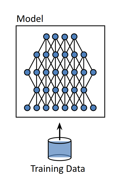
The need to train increasingle large models, some with billions of parameters, has necassitated a shift towards distributed training across multiple GPUs. This shift is driven by the fact that many advanced models cannot fit into memory of a single GPU. Instead, distributing the computational workload across sevaral GPUs offers a feasible solution. The practive of distributed training gained traction when CNNs were being trained on large datasets like ImageNet. In such networks, the initial convolutional layers are particularly computation-intensive due to the stencil operation required to process the entire image. This realization led to early efforts in distributed training focusing primarily on dividing the compute heavy tasks among multiple GPUs. This kind of splitting model parameters across multiple GPUs is called model parallelism.
parallelism in deep learning perspective is of the following types:
- model parallel
- data parallel
- tensor parallel
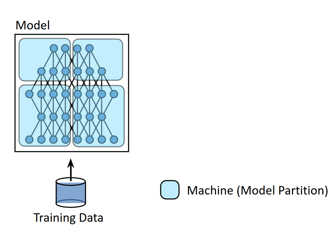
model parallel is the easiest to implement as we dont have multiple replicas of the same parameter and no reduction is required. The only change required from the normal training routine is at some point the intermediate outputs need to be transferred from one GPU to the other.
Data Parallelism#
data parallelism is a cornerstone of distributed training strategies, especially when dealing with extensive deep learning models. In this approach, each GPU holds a complete copy of the model, ensuring that every unit can independently process different subsets of the overall dataset. While this method effectively utilizes the parallel nature of GPUs, it introduces significant complexity during the backward pass, particularly in gradient accumulation and synchronization.
The challenge arises from the need to integrate gradients computed induvidually on each GPU. Since different GPUs process different data, the generate unique gradients, which must be averaged before updating the model’s weights. This averaging is crucial because it ensures that the model learns uniformly from the entire dataset rather than just fragments of it.
There was a trick used to train models of larger batch size than possible using gradient accumlation, this method computes gradients every batch but only updates the weights interleaved.
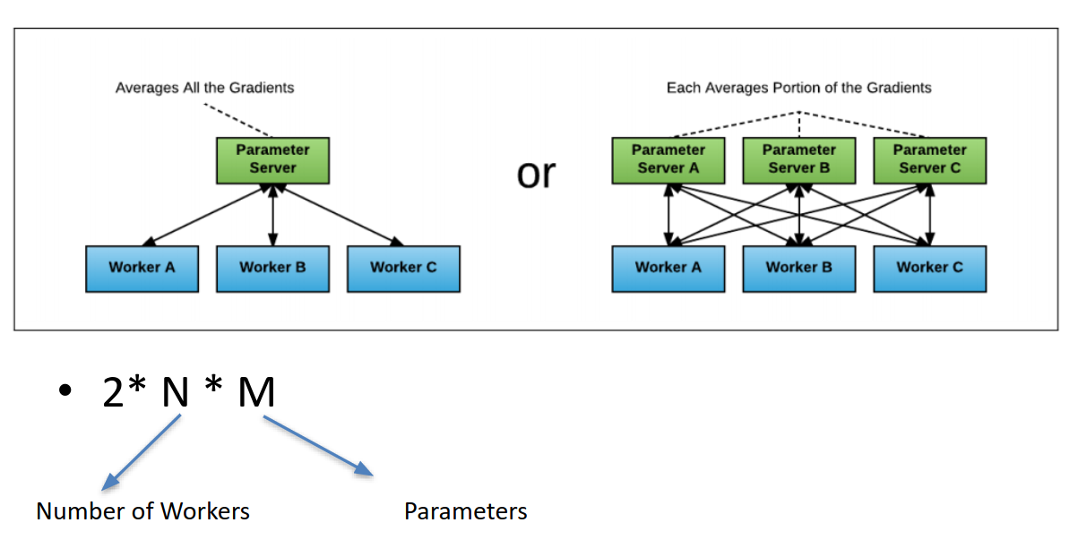
Several methods are employed to manage this averaging process across machines. A commonly used technique involves a parameter server architecture. In this setup, a central server aggregates the gradients from all GPU’s. This method, however has scalability limitations. As the number of GPUs increases often going beyond ten the parameter server can become a bottleneck, straining under the heavy load of receiving and processing gradients from each unit. This can potentially halt the training process, affecting efficiency and scalability.
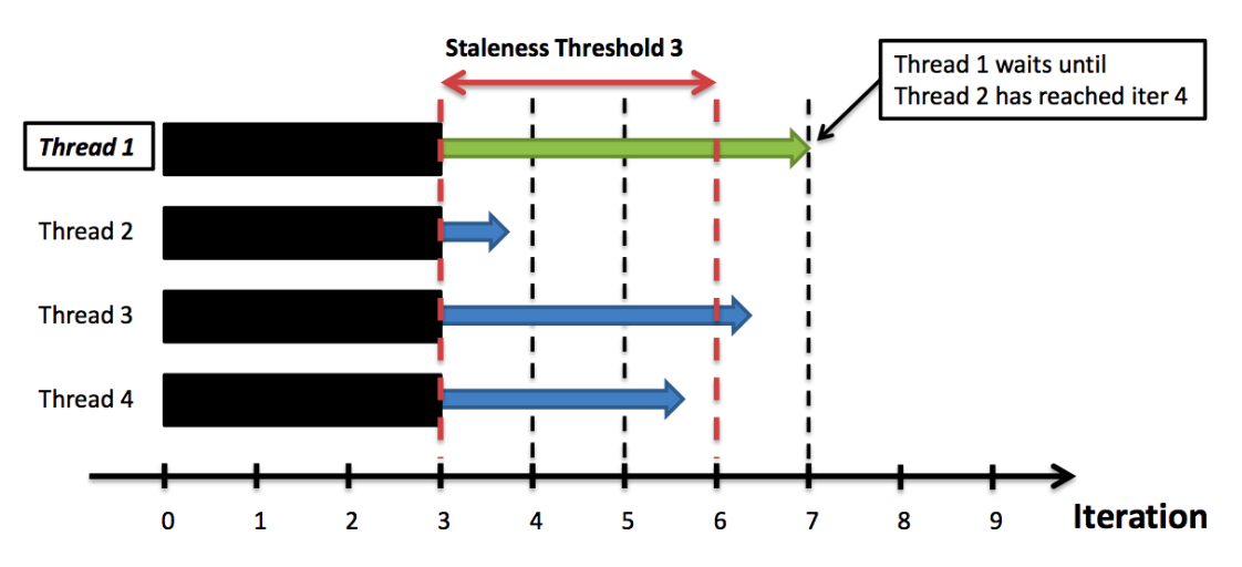
Frameworks like tensorflow have addresed some of these issues by implementing advanced versions of the parameter server model, which are designed to handle large clussters more effectively. In addition to the challenges of gradient averaging, data parallelism must also manage synchronization issues that arise when nodes vary in computational speed. This variation can introduce a problem known as staleness, where the updates from slower nodes lag behind those from faster ones.
During a distributed training session, each GPU (or node) processes a different batch of data and computes gradients independently. Ideally, these gradients are synchronized across all nodes to update the model weights uniformly. However, if one node takes significantly longer to process its batch, it causes a delay in the aggregation of gradients. As a result, faster nodes must wait for the slower ones to finish computation, leading to idle time that can significantly reduce overall system efficiency.
There is additional overhead when dealing with fault tolerency in these synchronization, but that is beyond the scope of this discussion.
This staleness not only affect the synchronization step but can also impact the accuracy and convergence of the model. If gradients from slower nodes are outdated by the time they are integrated, they might not accurately represent the current state of the model leading to suboptimal updates.
To mitigate these issues, various synchronization strategies are employed. One common approach is to use barrier synchronization, where all nodes must reach a certain point in the computation before any of them can proceed. This ensures that all gradient updates are based on the same version of the model, preventing staleness. However this method can lead to increased waiting times, as all nodes are forced to operate at the pace of the slowest one.
Another approach is to implement asynchronous updates, where nodes update the central model with their gradients as soon as they are ready, without waiting for the slowest nodes. This mothod can improve the efficiency of the system by reducing idle time but at the cost of introducing more staleness into model updates, which can complicate convergence.
Despite These bottleneck issue can still pose significant challenges, prompting the development and adoption of more sophisticated techniques such as ring-allreduce. This method distributes the task of gradient aggregation across all devices, therby eliminating the need for a central parameter server and significantly reducing the communication overhead.
Horovod#
Horovod is a distributed training framework introduced by Uber by modifying the common ring-reduce algorithm this significantly enhances the efficiency of data synchronization across multiple GPUs by employing the ring allreduce algorithm. This method is specifically designed to minimize the communication overhead by reducing the number of simultaneous data transfers, thus avoiding bandwidth saturation and ensuring a stable and fast data exchange.
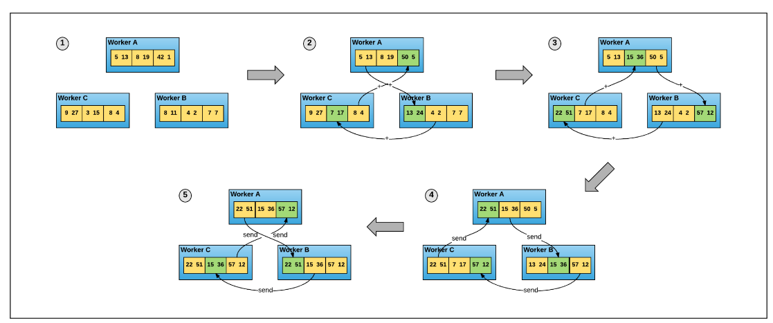
The ring-allreduce algorithm operates by organizing each GPU into a virtual ring topology. It begins by dividing the gradient data into equal segments and assigning each segment to a GPU. In this setup, each node is responsible for sending a segment of its data to its neighbor on the right and simultaneously recieving a segment from its neighbor on the left. Upon recieving a segment, a node quickly combines it with its correspponding segment a process known as reduction. After reducing the data, the node passes the resultant data to the next node in the ring. This process of rotating and reducing continues until every segment has circulated back to its original node.
By the end of this cyclem each GPU has recieved segments of data from all other GPUs, ensuring that each segment is fully reduced set of gradients from across the network. These averaged gradients are then used to update the model weights on each GPU, synchronizing the model state across all nodes to maintain uniformly for the next training iteration.
One of the primary benifits of horovod is its efficient use of network resources. The framework manages to distribute the communication load evenly across all participating GPUs. By transferring the weights in a round-robin fashion and processing the data in manageble parts, Horovod stays within the available bandwidth limits. This careful management helps in reducing network congestion and ensures a smoother gradient averaging process making horovod particularly advantageous in environments where network resources are constraint.
Exploring PyTorch’s Approach to Distributed training#
Pytorch offers a robust distributed training framework that differs notably from Horovod’s methodology. Unline Horovod, which synchronizes gradients after they are computed across all GPUs Pytorch synchronizes gradients as soon as they become available, facilitating a more dynamic and efficient workflow. This immediate synchronization is part of PyTorch’s Distributed Data Parallel (DDP) architecture, which is designed to enhance performance, particularly in environments where bandwidth might be a limiting factor [it always is].
The key to Pytorch’s efficiency lies in its ability to overlap gradient computation with gradient synchronization. Here’s how this process typically unfolds: pytorch groups gradients into what are called buckets. as soon as one of these buckets are filled with computed gradients, it doesn’t wait for the rest of the model to finish computing its gradients. Instead it immediately begins the synchronization process for that bucket. This method allows DDP to initialize the communication phase much earlier than if it had to wait for the entire backward pass to complete.
This overlapping of computation and communication is highly benificial. It ensures that the GPUs are not left idle waiting for data, thus making full use of the network bandwidth and reducing overall training time. By starting the synchronization process as a portion of the gradients is ready, pytorch minimizes the downtime that each GPU might otherwise experience if it had to wait for the entire network’s gradients to be computed befire beginning synchronization.
Pytorch provides two common methods are used to facilitate the training of deep learning models across multiple GPUs: Data Parallel (DP) and Distributed Data Parallel (DDP). While both approaches aim to distribute the training workload across several computing units, They are fundamentally different in how they manage and execute this distribution.
Distributed Data Parallel (DDP):#
Distrbuted Data Parallel, is optimized for both single machine and multi machine configurations. DDP improves upon the basic idea od DP by reducing the communication bottleneck observed in DP. It does this by eliminating the need for a master GPU. Instead, each GPU independently computes the gradients from its subset of the data, and then a collective communication operation (like all-reduce) is employed to average these gradients across all devices without funneling through a single point. DDP uses processes instead of theads for handling parallel tasks across multiple GPUs. This design choice is pivotal for enhancing performance and avoiding common pitfalls associated with multithreading in python, such as Global Interpreter Lock (GIL) constraints. Additionally, processes improve scalability across varied hardware and network architectures. They support robust and reliable communication mechanisms, such as NCCL, MPI. These are specifically optimized for inter process communication, enhancing the overall efficiency and effictiveness of distributed training operations.
Some Key words of DDP are:#
- WORLD_SIZE: defines the total number of workers n1 nodes n2 gpus = n1 * n2
- WORLD_RANK: identifies the worker ranges from 0..(n1*n2)
- LOCAL_RANK: defines the id of a worker within a node or indirectly refers to the gpu rank